This case study examines methods of assessing how C-ITS can deliver specific benefits for dedicated freight operations between Nissan (NMUK) and Port of Tyne, notably time savings, fuel savings and emission reductions.
Cooperative Intelligent Transport Systems (C-ITS) facilitate real-me communication between vehicles
and infrastructure, enhancing overall traffic management, safety, and environmental priorities.
This case study explores the potential impacts of C-ITS deployment on NMUK logistics operations to and
from the Port of Tyne (PoT). In surveying the characteristics of this vital strategic corridor, it is possible to
assess the benefits accruing from C-ITS on fuel consumption, emissions, and journey me savings.
Transport and logistics are of significant importance to the North East region. The region has 5 ports and
an international airport, major cities, and is home to Nissan (the UK’s largest manufacturing plant) and a
significant number of automotive supply chain businesses. The logistics industry requires innovative
solutions that can enhance efficiency and control cost competiveness, while reducing environmental
impact. Emissions from HGVs are a significant concern, as they are a major contributor to air pollution
and climate change.
It is anticipated that the insights from this case study will contribute to more detailed feasibility studies
or funded research that make a mely and significance contribu on to evidence-led logistics industry
practice and policy, supporting the adoption of advanced technologies for more sustainable logistics
operations. The implications may extend beyond NMUK and PoT, informing policymakers and logistics
operators on strategies for creating more sustainable and efficient transportatition networks.
The problem to be solved is reduction in fuel consumption and emissions by eliminating stops at red
traffic signals using C-ITS. Journey time reliability could also be improved. Benefits are cost savings and
efficiency improvements for stakeholders.
A vehicle’s fuel consumption is determined by distance travelled, topography, vehicle-related (fuel, age,
loading) and driver behaviour-related (speed, braking, acceleration) factors.
The process of stopping at a red traffic signal consists of deceleration to a stop, idling while stationary,
and acceleration to road speed. These actions contribute to an increase in fuel consumption and
emissions, thus measures to reduce the number of signal stops can achieve fuel savings. The fuel
consumption in terms of volumetric flow from stopping at one traffic light is as follows [1, 2]:
• Deceleration consumes 1.81 Lh-1
• Idling consumes around 0.9-1.3 Lh-1, (1.24 Lh-1 for HGVs specifically)
• Acceleration consumes 9.80 Lh-1
For this PCS, current fuel consumption of HGVs can be calculated from data provided by NMUK’s logistics
partner BCA. Fuel savings can then be determined from the number of stops (and thus decelera>onidling-
acceleration actions) that are eliminated through deployment of C-ITS. An associated reduction in
emissions can also be calculated.
[1] Chen C., Huang C., Jing Q., Wang H., Pan H., Li L., Zhao J., Dai Y., Huang H., Schipper L. and Streets D.G.
(2007), On-Road Emission Characteristics of Heavy-Duty Diesel Vehicles in Shanghai. Atmospheric
Environment (2007), 41, 5334-5344.
[2] Hlasny T., Fanti M.P., Mangini A.M., Rotunno G., Turchiano B. (2017), Optimal Fuel Consumption for
Heavy Trucks: A Review. IEEE Interna>=tional Conference on Service Operations and Logistics, and
Informatics (SOLI), 30 November 2017 Bari, Italy. IEEE.
What is the solution to the problem?
Cooperative Intelligent Transport Systems (C-ITS)
Intelligent Transport Systems (ITS) leverage technologies to develop intelligent infrastructure, vehicles,
and users to enhance efficiency, comfort, safety, and environmental sustainability. Advancements in
wireless communications have paved the way for the emergence of Coopera>ve (or Connected)
Intelligent Transportation Systems (C-ITS). These leverage wireless connectivity (4G or 5G) between
vehicles and infrastructure to enable cooperative interactions and information exchange.
It is important here to differentiate between two common types of C-ITS service:
• Green Light Optimal Speed Advisory (GLOSA). Information is provided to the vehicle’s driver,
allowing him/her to take action to implement a fuel-optimal trajectory to signals
• Green Priority. Communication takes place between the vehicle and urban traffic management
centre (UTMC) to attenuate a traffic signal, with no information provided to, and therefore no action
required of, the driver. It can extend an existing green signal phase or hurry a future phase for the
vehicle, enabling creation of ‘green waves’
The DSIT 5G IR project deploys a green priority system using rtip onboard units on selected buses in
Sunderland. This utilises the 5G network to improve the C-ITS solution to amenuate the infrastructure –
i.e. the traffic signal - rather than the bus speed. The overall aim is to improve journey time reliability by
reducing actual and perceived delays from signals, whilst ensuring minimum disrup>on to other traffic
streams and creating green waves for late running vehicles.
The 5G IR project also investigates, in this PCS, the potential for a C-ITS service to be deployed for HGVs
on a specific route from NMUK to the Port of Tyne. The researchers remain agnostic about the most
appropriate service. The key is to examine the poten>al impact of a C-ITS service fuel consumption,
journey time, and emissions through elimination of traffic signal stops.
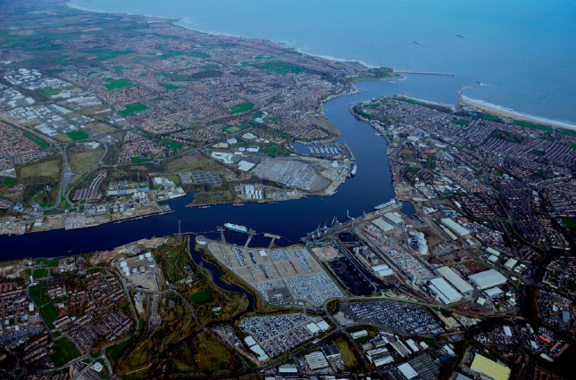
The Route
The research team drove the route to identify number and location of traffic signals, length of journey,
total time taken, and speeds on each section. Automated data collection included video of the route to
obtain locations and number of stops and to record weather and traffic levels; GPS data (GeoTracker
Android App) tracked stops, speeds, and acceleration. To obtain the number of stops at red signals and
time held, the route was driven 8 times in both directions to obtain averages: outbound trips to the Port
of Tyne (1A-8A) and inbound trips (1B-8B). A portion of the route encompasses private roads at NMUK
and the Port of Tyne however, the PCS focuses on the public road segments (Figure 1). The three main
roads on this route are A1290, A19, A185. There are no traffic signals on the A19.
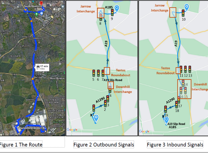
There are 9 signals outbound (A trips), and 11 inbound (B Trips) (Figure 2 and Figure 3). The traffic signal
when exiting the Port of Tyne (#10 in Figure 3) is excluded as it always requires a stop, therefore the test
route only includes 10 signals inbound.
Commercial model (Business Case)
Stopping Data
Stopping data for each traffic signal was obtained from the video footage for all trips. Across the 8 round
trips (outbound and inbound), some signals did not cause the vehicle to stop even once (these were
pedestrian crossings (3, 7, 8, 9, 10, 13, 17 in Figures 2 and 3)). Time values include the time taken to
decelerate, the idling time, and the time taken to accelerate back to road speed. This method was applied
to all 8 trips, allowing the percentage of time spent at signals to be derived. Using percentages bemer
represents the total length of the journey, rather than just an absolute time value.
The average percentage of journey time spent at signals was 13.12% for outbound trips and 11.3% for
inbound trips.
Journey and Vehicle Data
The fleet consists of 12 diesel vehicles, all of which are Volvo FM rigid trucks with ROLFO Sirio H trailers.
Each vehicle performs 14 complete circuits every day, which is equal to 28 single journeys (combining
inbound and outbound trips). There are approximately 48 plant production weeks in a year. This data
enabled the team to extrapolate data for one vehicle stopping at one signal across the whole fleet and
multiple timeframes.
Benefits
Assessment of the Benefits of C-ITS
In an optimistic case scenario, there would be no stops at any of the traffic signals on the route. However,
Signal 1 and Signal 19 (Figures 2 and 3) are situated at a T-junction. This means that vehicles would
significantly slow down at this junction, regardless of a red signal, due to the geometry and tightness of
the road. Therefore, it is presumed that C-ITS cannot be deployed at this junction.
From the data collected on the 8 runs, the average number of stops is 3.00 for outbound A trips, and
3.375 for inbound B trips. In an optimistic case, none of these stops would occur. During the test drives,
the vehicle stopped at Signal 1 every time and at Signal 19 four out of eight times (50%). Therefore, if CITS
is not to be deployed at these signals, the average number of stops can be reduced by 1.00 for A Trips
and by 0.50 for B Trips. Throughout the analysis of C-ITS benefits, these two case scenarios will be
consistently referred to as OCS (Optimistic Case Scenario) – where all outbound and inbound stops are
eliminated - and RCS (Realis>c Case Scenario) – where all are eliminated bar Signals 1/19.
Lessons Learnt
Summary of Methods
In the accompanying report, three methods are described for analysing fuel consumption and emissions
savings.
For Method 1 (described above), the time spent at a traffic signal is split into three phases, replicating
the acceleration-deceleration profile: 60% of this time is spent in acceleration, 30% in deceleration, and
10% idling. Multiplying these times by the respective fuel consumption rates for each phase yields the
total fuel consumed during one stop. The savings are approximately 1.75% in OCS and 1.19% in RCS.
Associated emissions reductions are calculated by applying conversion factors.
Method 2 offers insights into HGVs specifically, utilising a fuel consumption rate of 0.12 litres per stop,
from a study by [4]. This method also yields fuel and emissions savings, but it overlooks the braking accelera
tion process.
Given that the HGVs utilised by Nissan are notably larger and heavier than the test vehicle, a Vauxhall
Corsa, it is expected that they would require more time to come to a stop and subsequently accelerate
back to their original speeds. Method 3 addresses this limitation by expanding on Method 1 to analyse
the deceleration-acceleration profile of a double-decker bus; this is more akin to the distinctive
deceleration and acceleration pamerns inherent to HGVs.
Method 3 is the preferred choice due to the double-decker bus more closely approximating HGV
characteristics. By accounting for the longer duration and unique characteristics of HGVs during stop-go
manoeuvres, a more accurate estimations of fuel consumption and emissions savings is obtained. For
optimistic scenarios (OCS), the projected reduction in journey times is at least 12.34%, with associated
savings of 5.26% for fuel and emissions. This translates to approximately 27.2 kilolitres or 53.2 tonnes
CO2e annually. In more realistic scenarios (RCS), the expected reduction in journey times is at least 9.21%,
with corresponding savings of 3.56% for fuel and emissions. This equates to around 18.5 kilolitres and 36
tonnes CO2e annually.
Full analysis of all three methods is presented in the accompanying report.
Assumptions/Limitations
• Data Collection Limitations
o Limited number of test drives conducted (only 8 complete journeys)
o Test drives were conducted within a specific time frame, between 11:30am and 2:30pm,
potentially limiting the representation of different traffic conditions
o The test vehicle used was a car, which may not accurately reflect the speed and
performance characteristics of HGVs
• Data Analysis Limitations
o Variations of running laden conditions of HGVs were not fully accounted for in the
analysis
o The effectiveness of C-ITS and the exact number of eliminated stops are estimated rather
than precisely measured
o The heavy vehicle acceleration profile used in Method 3 is based on data from a doubledecker
bus, which may not fully represent the acceleration characteristics of HGVs
[4] Deschle N., Van Ark E.J., Van Gijlswijk R. and Janssen R. (2022), Impact of Signalized Intersections on
CO2 and NOx Emissions of Heavy Duty Vehicles. Energies (Basel), 15, 1242.
If you’re ready to embark on a connectivity project, we can point you to the suppliers with expertise in your sector.